Infomax Independent Component Analysis for Dummies
Introduction
Independent Component Analysis is a signal processing method for separating independent sources that have been linearly mixed across several sensors. For example, when recording electroencephalograms (EEG) on the scalp, ICA can often separate artifacts and neural activity when their statistical structure is sufficiently distinct and approximately independent, though exact independence is not required and separation is not guaranteed.
This page explains ICA to researchers who want to understand it but have only a modest background in matrix computation and information theory. The explanations are as intuitive as possible and based on practical Matlab examples.
You may also find this series of videos helpful (in particular video 3), which gives detailed explanations on how to apply ICA to EEG data.
What is ICA?
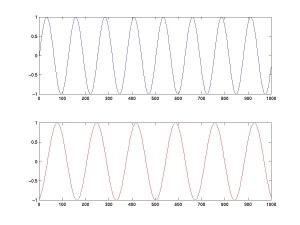
ICA separates linearly mixed sources. For instance, let's mix and then separate two sources. We define the time courses of two independent sources, A (top) and B (bottom). (Matlab code | Python code)
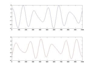
We then mix these two sources linearly. The top curve equals A minus twice B; the bottom is the combination 1.73×A + 3.41×B.
We feed these two signals into an ICA algorithm (here, FastICA), which recovers the original activations of A and B.
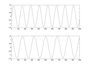
Note that the algorithm cannot recover the exact amplitude of the source activities (we will see why later). Performance often remains reasonable at moderate noise levels, but robustness depends on the signal-to-noise ratio, model mismatch, sample size, and algorithm settings. Also note that, in theory, ICA can only extract sources that are combined linearly.
Whitening the data
A first step in many ICA algorithms is to whiten (or sphere) the data. This means removing any correlations so that the different channels are forced to be uncorrelated.
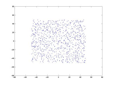
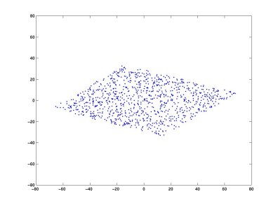
Why do that? Geometrically, whitening removes second-order correlations and rescales the data so that the covariance becomes the identity. After whitening, ICA estimates an additional transformation, often described in the simplified two-dimensional case as a rotation. Let's mix two random sources A and B. In the scatter plot below, each data point's x-coordinate is the value of A and its y-coordinate is the value of B.
Taking two linear mixtures of A and B (Matlab code | Python code) and plotting the two new variables:
After whitening the two mixtures:
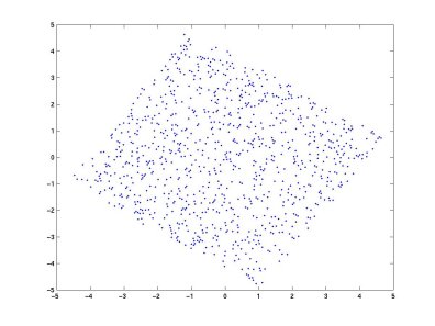
The variance on both axes is now equal, and the correlation between the two projections is zero (the covariance matrix is diagonal with equal elements). In the simplified whitened two-dimensional case, ICA can be viewed as finding a rotation that aligns the axes with the source directions.
Whitening is simply a linear change of coordinates. Once ICA finds its solution in the whitened frame, it is straightforward to reproject back into the original coordinate frame.
The ICA algorithm
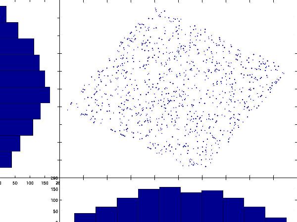
Intuitively, ICA rotates the whitened data back to the original (A, B) space. After whitening, many ICA algorithms estimate components by finding directions whose projections are maximally non-Gaussian, or equivalently by optimizing related criteria such as negentropy, likelihood, or mutual information under specific assumptions. In the whitened scatter plot, the projections onto both axes are fairly Gaussian (bell-shaped):
By contrast, projections in the original A, B space are far from Gaussian:
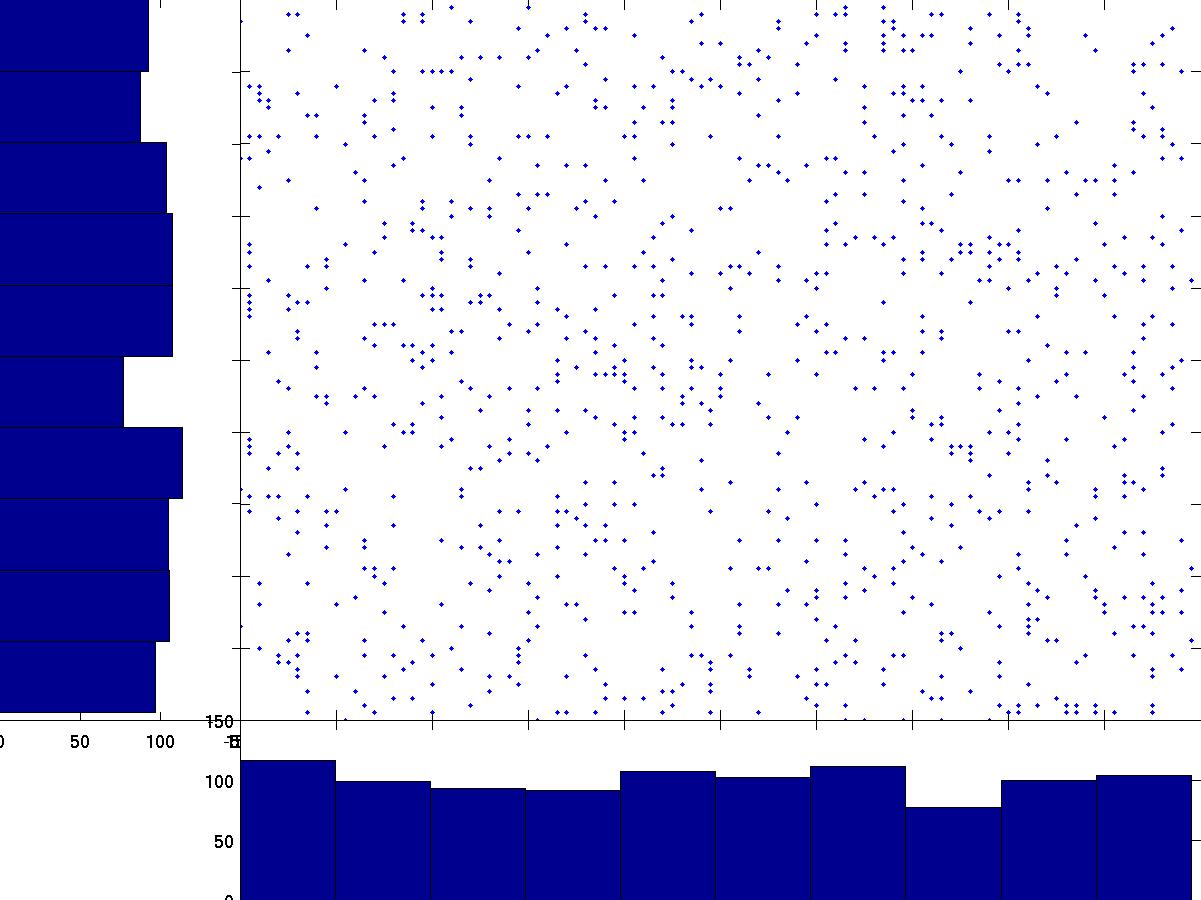
By rotating the axes to minimize Gaussianity, ICA recovers the original sources that are statistically independent. This works because, under standard ICA assumptions, a linear mixture of independent non-Gaussian variables tends to be more Gaussian than the original sources. This intuition follows from the central limit theorem.
In Matlab, the function kurtosis (kurt() in the EEGLAB toolbox;
kurtosis() in the Statistics Toolbox) gives an indication of Gaussianity.
The FastICA algorithm uses a slightly different measure called negentropy.
The Infomax ICA algorithm in the EEGLAB toolbox works by minimizing the mutual information of the projected components. Although many ICA algorithms are closely related, they are not all theoretically equivalent. Different algorithms optimize different objective functions and may yield different decompositions depending on the source model and data.
ICA in N dimensions
So far we have worked with only two dimensions, but ICA handles arbitrarily high dimensionalities. Consider 128 EEG electrodes: the signal recorded at all electrodes at each time point forms a data point in 128-dimensional space. After whitening, many ICA methods estimate component directions by optimizing statistical independence or non-Gaussianity. In the whitened space this is often represented as an orthogonal transform, whereas the corresponding filters in the original data space need not be orthogonal.
Each ICA component is a projection from the original data space onto one of the axes found by ICA. The full transformation is captured by the weight matrix. When we write:
X is the data in the original space. For EEG, each row is an electrode and each column is a time point:
                t1      t2      t3      t4      t5      t6      t7
Electrode 1   [  0.968  -0.067  -0.224   1.175   0.395  -0.583   0.562 ...]
Electrode 2   [  0.132   1.164   0.397  -0.034   1.014  -0.536  -0.558 ...]
Electrode 3   [ -0.436  -0.275   1.069   0.321  -0.185   1.051  -0.158 ...]
For fMRI, the convention is transposed: each row is a time point and each column is a voxel.
S is the source activity matrix. Each row is the time course of one independent component—which may represent an artifact or a compact cortical source:
                t1      t2      t3      t4      t5      t6      t7
Component 1   [  0.820   0.530  -0.310   0.650   0.740  -0.930   0.180 ...]
Component 2   [ -0.410   0.720   0.930  -0.180   0.530   0.340  -0.650 ...]
Component 3   [  0.150  -0.640   0.470   0.830  -0.290   0.610   0.380 ...]
W is the weight matrix. Each row of W is the spatial filter for one component: multiplying that row by the data matrix X yields the component's time course.
                  elec1   elec2   elec3
Component 1   [  0.650   0.420  -0.310 ]
Component 2   [ -0.280   0.730   0.540 ]
Component 3   [  0.510  -0.360   0.680 ]
For instance, to compute the activity of the second independent component, multiply its row of W by the data matrix X:
Component 2 [ -0.280 0.730 0.540 ]
The component activity is unitless until projected back to electrode space. This is analogous to equivalent dipoles in source localization: each dipole has an activity that projects linearly to all electrodes.
Projecting back to sensor space
W−1 is the inverse weight matrix. The back-projection is:
In Matlab, inv(W) gives the inverse. Each column of
W−1 is the scalp topography of one component:
                 comp1   comp2   comp3
Electrode 1   [  0.948  -0.239   0.622 ]
Electrode 2   [  0.639   0.823  -0.363 ]
Electrode 3   [ -0.373   0.615   0.812 ]
To obtain the contribution of a single component (say component 2) to the data, multiply its inverse-weight column vector by its activity row vector:
Electrode 1   [ -0.239 ]
Electrode 2   [  0.823 ]
Electrode 3   [  0.615 ]
Multiplying this column vector (left) by the component 2 activity row vector (top) gives the full projection XC2—a channels × time-points matrix:
                t1      t2      t3      t4      t5      t6      t7
              [ -0.410   0.720   0.930  -0.180   0.530   0.340  -0.650 ...]

[ -0.239 ]    [  0.098  -0.172  -0.222   0.043  -0.127  -0.081   0.155 ...]
[  0.823 ]    [ -0.338   0.593   0.766  -0.148   0.436   0.280  -0.535 ...]
[  0.615 ]    [ -0.252   0.443   0.572  -0.111   0.326   0.209  -0.400 ...]
To remove an artifact component from the data, simply subtract its projection:
Because all columns of XC2 are proportional, the columns of W−1 represent the scalp topography of each component—a fixed spatial pattern that is scaled in time by the component activity. This scalp topography is often used as an input to equivalent dipole fitting for putative brain components, although a good dipole fit is model-dependent and does not by itself prove a single focal cortical source.
- Rows of S—the time course of each component's activity.
- Columns of W−1—the scalp topography of each component.
ICA of EEG data
The earlier sections used idealized sources with flat (maximum-entropy) probability density distributions. In practice, EEG sources have peaky, super-Gaussian distributions. We use a non-linear function to transform these distributions into ones for which we can maximize entropy. This is explained in detail in this video.
ICA properties
- ICA can only separate linearly mixed sources.
- For standard instantaneous ICA applied to samples without using temporal structure, permuting time points has little or no effect on the outcome. This statement does not necessarily hold for ICA variants or preprocessing steps that exploit temporal information.
- Changing channel order does not change the decomposition apart from the corresponding permutation of the mixing and unmixing matrices, provided the same data are otherwise used. ICA has no a priori knowledge of electrode locations; the observation that some ICA component scalp maps are well fit by a single equivalent dipole is consistent with, but does not by itself prove, a compact underlying generator.
- In linear ICA, Gaussian sources are problematic for identifiability. In particular, if more than one source is Gaussian, the Gaussian subspace cannot in general be uniquely separated.
- Even when sources are not truly independent, ICA finds a space in which they are maximally independent.
Annex: the math behind whitening
We seek a linear transformation V of the data D such that when P = VD, we have Cov(P) = I (the identity matrix). This means all rows of the transformed matrix are uncorrelated.
Let Z be the centered version of D. Then Cov(D) = Cov(Z) = ZZ'/(n−1).
Setting V = C−1/2, where C = Cov(D), gives:
Computing Cx is non-trivial; it is defined such that Cx C−x = I and involves eigendecomposition of the covariance matrix.